
California housing prices
Table of Contents:
Preprocessing the data
#importing the libraries
import os
import numpy as np
import pandas as pd
import seaborn as sns
import matplotlib.pyplot as plt
#loading the dataset and obtaining info about columns
df=pd.read_csv("housing.csv")
list(df)
['longitude',
 'latitude',
 'housing_median_age',
 'total_rooms',
 'total_bedrooms',
 'population',
 'households',
 'median_income',
 'median_house_value',
 'ocean_proximity']
#description of the numerical columns
df.describe()
| longitude | latitude | housing_median_age | total_rooms | total_bedrooms | population | households | median_income | median_house_value | |
|---|---|---|---|---|---|---|---|---|---|
| count | 20640.000000 | 20640.000000 | 20640.000000 | 20640.000000 | 20433.000000 | 20640.000000 | 20640.000000 | 20640.000000 | 20640.000000 |
| mean | -119.569704 | 35.631861 | 28.639486 | 2635.763081 | 537.870553 | 1425.476744 | 499.539680 | 3.870671 | 206855.816909 |
| std | 2.003532 | 2.135952 | 12.585558 | 2181.615252 | 421.385070 | 1132.462122 | 382.329753 | 1.899822 | 115395.615874 |
| min | -124.350000 | 32.540000 | 1.000000 | 2.000000 | 1.000000 | 3.000000 | 1.000000 | 0.499900 | 14999.000000 |
| 25% | -121.800000 | 33.930000 | 18.000000 | 1447.750000 | 296.000000 | 787.000000 | 280.000000 | 2.563400 | 119600.000000 |
| 50% | -118.490000 | 34.260000 | 29.000000 | 2127.000000 | 435.000000 | 1166.000000 | 409.000000 | 3.534800 | 179700.000000 |
| 75% | -118.010000 | 37.710000 | 37.000000 | 3148.000000 | 647.000000 | 1725.000000 | 605.000000 | 4.743250 | 264725.000000 |
| max | -114.310000 | 41.950000 | 52.000000 | 39320.000000 | 6445.000000 | 35682.000000 | 6082.000000 | 15.000100 | 500001.000000 |
#count the values of the columns
df.count()
longitude             20640
latitude              20640
housing_median_age    20640
total_rooms           20640
total_bedrooms        20433
population            20640
households            20640
median_income         20640
median_house_value    20640
ocean_proximity       20640
dtype: int64
#We have missing values in the column total_bedrooms. We can drop the null rows or replace the null value for the mean.
#I choose to replace it with the mean
df['total_bedrooms'].fillna(df['total_bedrooms'].mean(), inplace=True)
#I want information about the column "ocean_proximity"
df['ocean_proximity'].value_counts()
<1H OCEAN     9136
INLAND        6551
NEAR OCEAN    2658
NEAR BAY      2290
ISLAND           5
Name: ocean_proximity, dtype: int64
#Transform the variable into a numerical one.
def map_age(age):
    if age == '<1H OCEAN':
        return 0
    elif age == 'INLAND':
        return 1
    elif age == 'NEAR OCEAN':
        return 2
    elif age == 'NEAR BAY':
        return 3
    elif age == 'ISLAND':
        return 4
df['ocean_proximity'] = df['ocean_proximity'].apply(map_age)
#Obtaining info of the correlations with a heatmap
plt.figure(figsize=(15,8))
corr = df.corr()
mask = np.zeros_like(corr, dtype=np.bool)
mask[np.triu_indices_from(mask)] = True
sns.heatmap(df.corr(), linewidths=.5,annot=True,mask=mask,cmap='coolwarm')
<matplotlib.axes._subplots.AxesSubplot at 0x2d174ac0eb8>
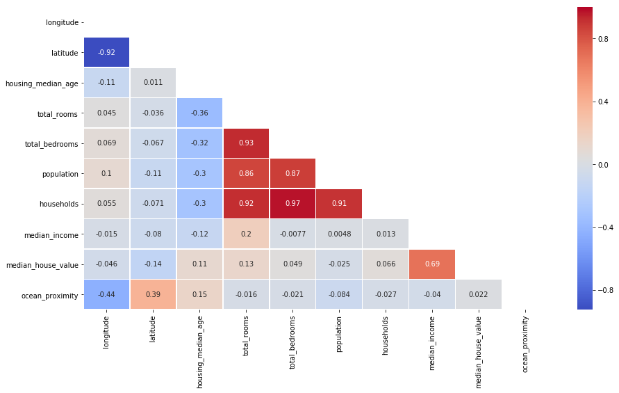
#There is a high correlation between households and population
df.drop('households', axis=1, inplace=True)
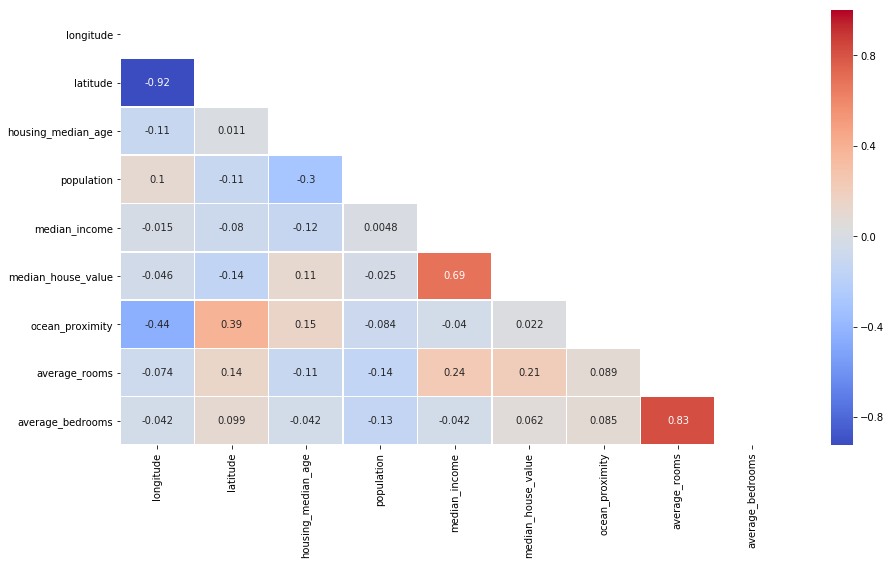
# let's create 2 more columns with the total bedrooms and rooms per population in the same block.
df['average_rooms']=df['total_rooms']/df['population']
df['average_bedrooms']=df['total_bedrooms']/df['population']
#dropping the 2 columns we are not going to use
df.drop('total_rooms',axis=1,inplace=True)
df.drop('total_bedrooms',axis=1,inplace=True)
#Obtaining info of the new correlations with a heatmap
plt.figure(figsize=(15,8))
corr = df.corr()
mask = np.zeros_like(corr, dtype=np.bool)
mask[np.triu_indices_from(mask)] = True
sns.heatmap(df.corr(), linewidths=.5,annot=True,mask=mask,cmap='coolwarm')
<matplotlib.axes._subplots.AxesSubplot at 0x2d1768818d0>
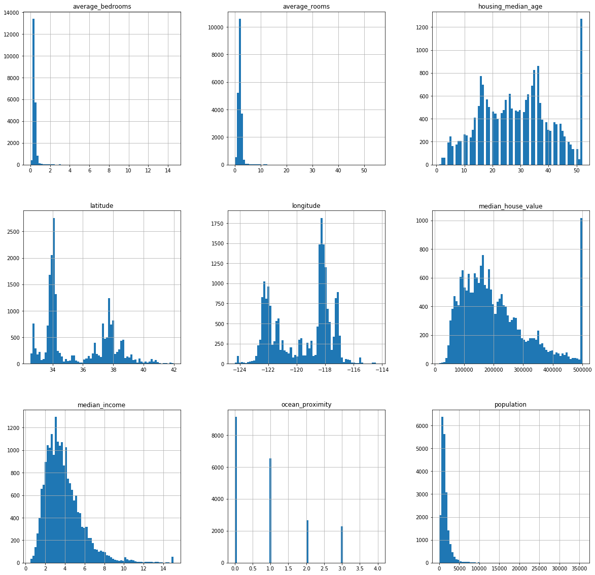
#histogram to get the distributions of the different variables
df.hist(bins=70, figsize=(20,20))
plt.show()
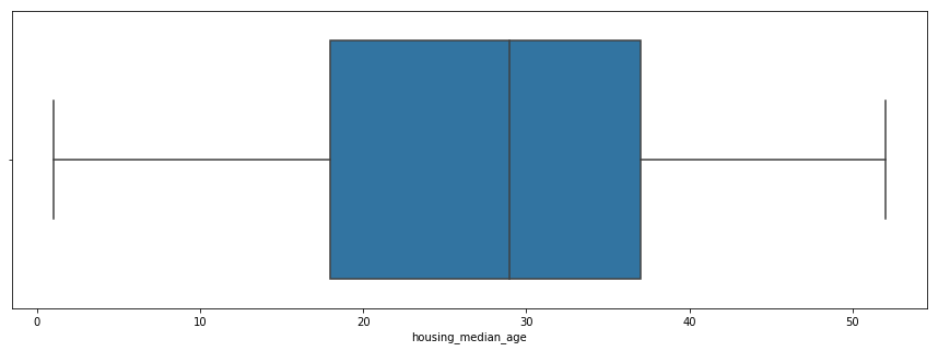
#Finding Outliers
plt.figure(figsize=(15,5))
sns.boxplot(x=df['housing_median_age'])
plt.figure()
plt.figure(figsize=(15,5))
sns.boxplot(x=df['median_house_value'])
<matplotlib.axes._subplots.AxesSubplot at 0x2d177c1d8d0>
<Figure size 432x288 with 0 Axes>
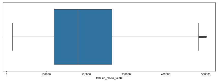
#removing outliers
df=df.loc[df['median_house_value']<500001,:]
Linear Regression
Training the model
#Choosing the dependant variable and the regressors. In this case we want to predict the housing price
X=df[['longitude',
 'latitude',
 'housing_median_age',
 'population',
 'median_income',
 'ocean_proximity',
 'average_rooms',
 'average_bedrooms']]
Y=df['median_house_value']
#splitting the dataset into the train set and the test set

from sklearn.model_selection import train_test_split
X_train,X_test,Y_train,Y_test = train_test_split(X,Y,test_size = 0.2, random_state=0)
#Training the model
from sklearn.linear_model import LinearRegression
regressor= LinearRegression()
regressor.fit(X_train,Y_train)
LinearRegression(copy_X=True, fit_intercept=True, n_jobs=None,
         normalize=False)
#Obtaining the predictions
y_pred = regressor.predict(X_test)
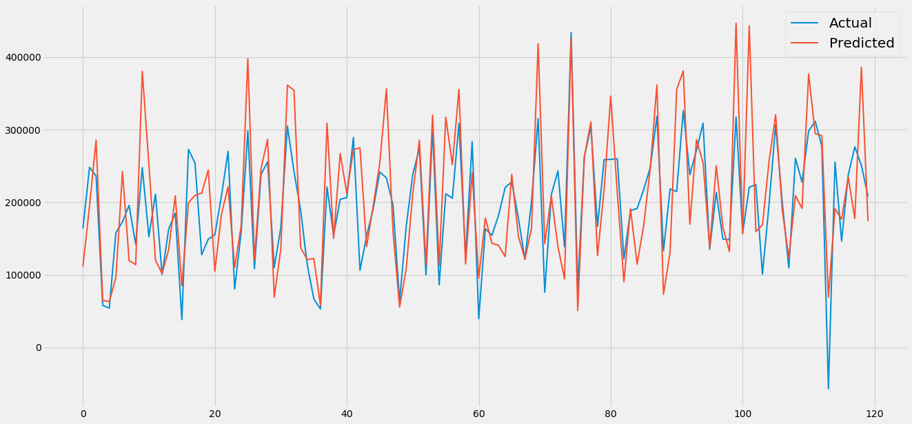
Evaluating the model
#R2 score
from sklearn.metrics import r2_score
r2=r2_score(Y_test,y_pred)
print('the R squared of the linear regression is:', r2)
the R squared of the linear regression is: 0.5526714001645363
#Graphically
grp = pd.DataFrame({'prediction':y_pred,'Actual':Y_test})
grp = grp.reset_index()
grp = grp.drop(['index'],axis=1)
plt.style.use('fivethirtyeight')
plt.figure(figsize=(20,10))
plt.plot(grp[:120],linewidth=2)
plt.legend(['Actual','Predicted'],prop={'size': 20})
<matplotlib.legend.Legend at 0x2d1765c9dd8>
XGBoost
Training the model
import xgboost as xgb
xg_reg = xgb.XGBRegressor(objective ='reg:linear', colsample_bytree = 1,eta=0.3, learning_rate = 0.1,
                max_depth = 5, alpha = 10, n_estimators = 2000)
xg_reg.fit(X_train,Y_train)

y_pred2 = xg_reg.predict(X_test)
Evaluating the model
#Graphically
grp = pd.DataFrame({'prediction':y_pred2,'Actual':Y_test})
grp = grp.reset_index()
grp = grp.drop(['index'],axis=1)
plt.figure(figsize=(20,10))
plt.plot(grp[:120],linewidth=2)
plt.legend(['Actual','Predicted'],prop={'size': 20})
<matplotlib.legend.Legend at 0x2d1783f10b8>
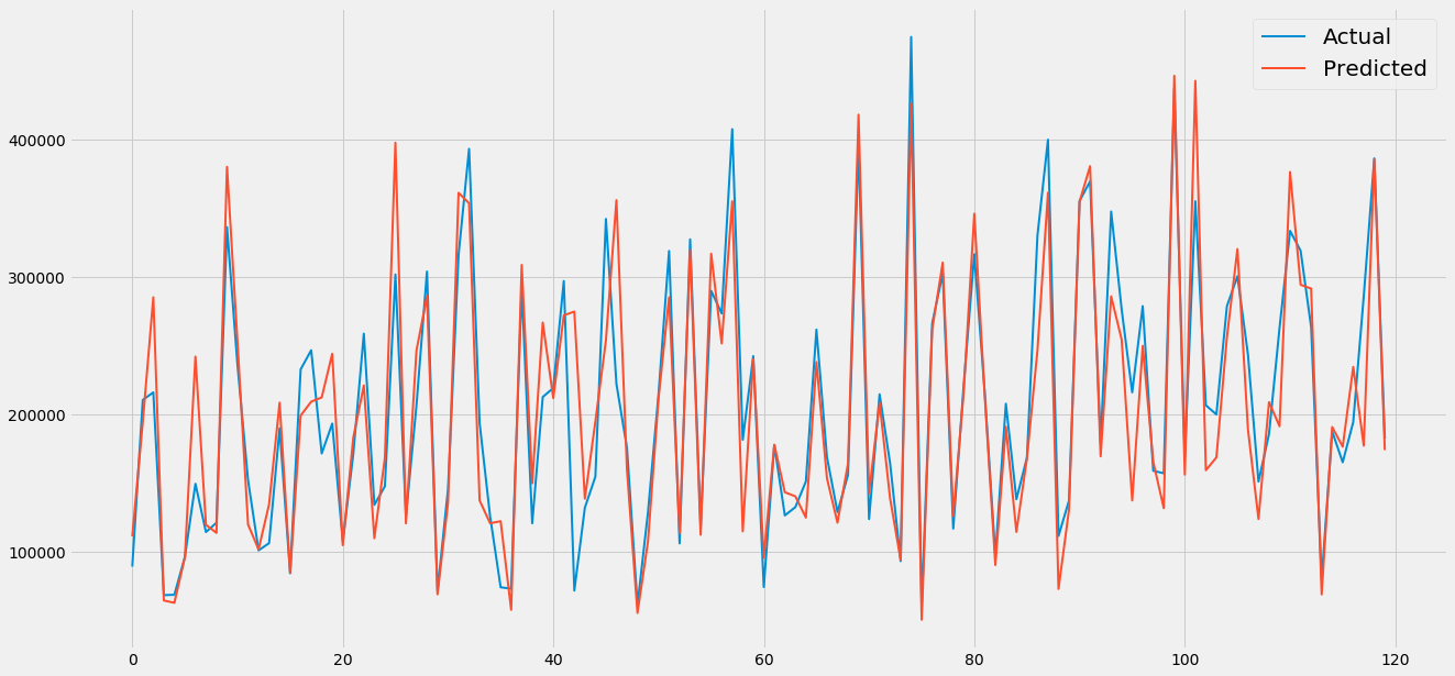
r2xgb=r2_score(Y_test,y_pred2)
print('the R squared of the xgboost method is:', r2xgb)
the R squared of the xgboost method is: 0.8227763364288538
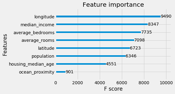
xgb.plot_importance(xg_reg)
plt.rcParams['figure.figsize'] = [5, 5]
plt.show()
#Doing cross validation to see the accuracy of the XGboost model
from sklearn.model_selection import KFold
from sklearn.model_selection import cross_val_score

kfold = KFold(n_splits=10, random_state=7)
results = cross_val_score(regressor, X, Y, cv=kfold)
print("Accuracy: %.2f%% (%.2f%%)" % (results.mean()*100, results.std()*100))
Accuracy: 43.75% (10.12%)
Linear regression vs XGBoost
#comparing the scores of both techniques
from sklearn.metrics import mean_squared_error
from sklearn.metrics import mean_absolute_error
from math import sqrt

mae1 = mean_absolute_error(Y_test, y_pred)
rms1 = sqrt(mean_squared_error(Y_test, y_pred))
mae2 =mean_absolute_error(Y_test,y_pred2)
rms2 = sqrt(mean_squared_error(Y_test, y_pred2))

print('Stats for the linear regression: \n','mean squared error: ',rms1, '\n R2:',r2,' \n mean absolute error:',mae1 )
print('Stats xgboost: \n','mean squared error: ',rms2, '\n R2:',r2xgb,' \n mean absolute error:',mae2 )
Stats for the linear regression:
 mean squared error:  65524.097680759056
 R2: 0.5526714001645363
 mean absolute error: 47427.66363813204
Stats xgboost:
 mean squared error:  41242.84075742074
 R2: 0.8227763364288538
 mean absolute error: 27488.045577549237